What Training Actually Means for a Transformer: Batches, Steps, and Epochs Explained
For about three years I couldn’t precisely answer this question: what does training a transformer actually mean?
Not in the handwavy “it learns from data” sense. In the operational sense — what computations run, in what order, how many times, and what changes as a result. This post is the answer I wish I’d had earlier.
The Textbook Analogy
Imagine you have a textbook with 10,000 sentences.
Training a transformer means:
- Show it a sentence
- Ask it to predict what comes next
- Check how wrong it was
- Nudge its internal weights to be a little less wrong next time
That’s the entire loop. The complexity isn’t in the idea — it’s in the mechanics of doing this at scale across billions of parameters and terabytes of data.
GPU Memory: Why You Can’t Feed It Everything at Once
You can’t show the model all 10,000 sentences in one go. Memory limits make that impossible.
When BERT was introduced in 2018, the most powerful widely-available GPU was the NVIDIA Tesla V100 — either 16 GB or 32 GB of HBM2 VRAM. Training BERT-Large (340M parameters) required multiple V100s running in parallel with gradient synchronization across them. Even with 32 GB per card, you cannot simultaneously hold the full dataset, the model weights, the optimizer states (Adam maintains two moment estimates per parameter), and the intermediate activations for the entire sequence.
So instead, you split the data into chunks. Each chunk gets processed, graded, and used to update the model. When you’ve gone through every chunk — every sentence in the book — that’s one full read-through of the data. That’s one epoch.
Before going further, it helps to have precise names for each piece.
The Four Levels: Batch, Step, Epoch, Training Run
Batch
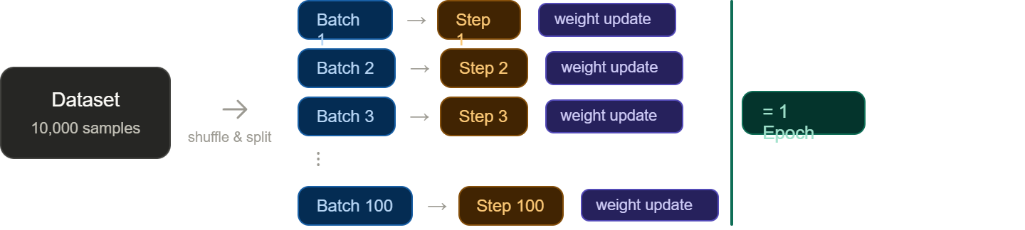
A batch is a subset of your dataset that fits in GPU memory and gets processed together.
If your dataset has 10,000 sentences and your batch size is 100, you have 100 batches.
Batch size is not a hyperparameter you set once and forget. Larger batches mean more stable gradient estimates but require more VRAM. Smaller batches introduce more noise into each weight update — which can sometimes help generalization — but are computationally less efficient per unit of data. In practice, batch size is often constrained by how much VRAM your hardware has, not by what would be mathematically ideal.
Step (Iteration)
A step, also called an iteration, is one complete cycle:
Take a batch → run it forward through the model → compute the loss → backpropagate gradients → update the weights
One batch = one step = one weight update.
Every time you hear “the model trained for 500 steps,” that means the weights were updated 500 times.
Epoch
An epoch is one complete pass through the entire dataset.
If you have 100 batches, then 100 steps = 1 epoch. After one epoch, the model has seen every training example exactly once.
Training Run
A training run is the entire process from start to finish — all epochs combined.
If you train for 5 epochs with 100 batches each: 5 × 100 = 500 total steps.
What Happens Inside a Single Training Step
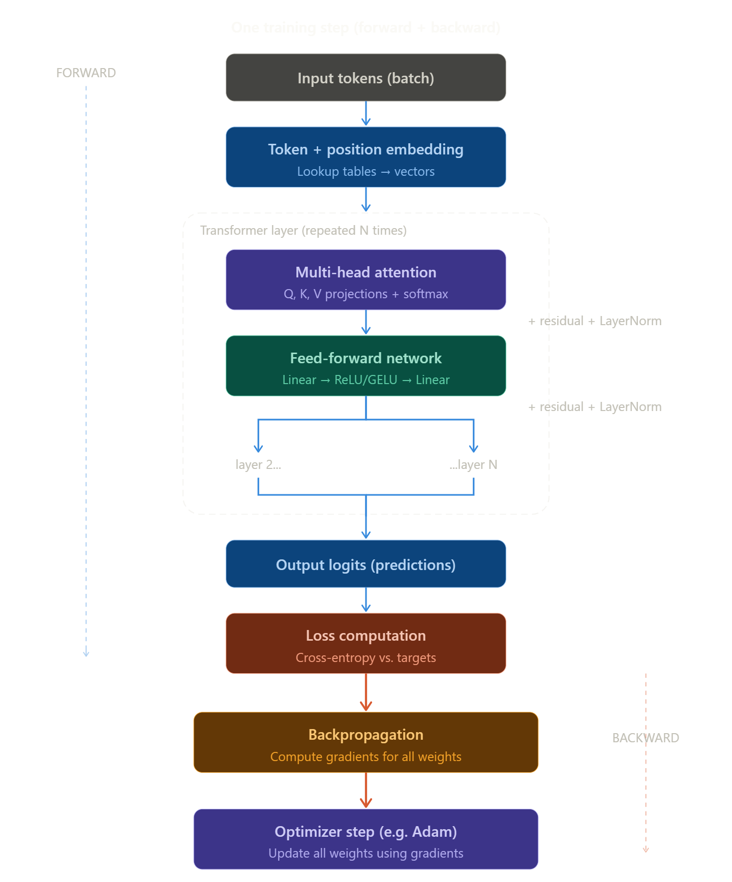
A step is not “the model reads a sentence.” A step is a full round trip through the entire model — forward, loss, backward, update.
Forward Pass (Blue Flow — Top to Bottom)
The batch of token IDs hits the embedding layer and becomes a matrix of vectors — one row per token, one column per embedding dimension.
These vectors pass through every transformer layer sequentially. Each layer applies two sublayers:
-
Multi-head self-attention — tokens “look at” each other to build context. Each token computes Query, Key, and Value vectors. The dot product of Q and K determines how much attention each token pays to every other token. The result is a weighted sum of V vectors — a contextually enriched representation. Multiple heads do this in parallel across different representation subspaces.
-
Position-wise feed-forward network (FFN) — each token independently passes through two linear transformations with a nonlinearity in between:
FFN(x) = max(0, xW₁ + b₁)W₂ + b₂. The FFN is where most of the model’s learned capacity lives.
After all N layers, the final representations are projected to vocabulary-sized logits — one probability distribution per token position, over every possible next token in the vocabulary. A softmax converts these logits into probabilities.
Loss Computation
The model’s predicted distribution is compared against the actual next tokens (for GPT-style autoregressive models) or the masked tokens (for BERT-style masked language models) using cross-entropy loss.
This produces a single scalar number: how wrong was the model on this batch?
Cross-entropy penalizes the model proportionally to how surprised it was by the correct answer. If the model assigned 90% probability to the right token, the loss contribution is low. If it assigned 1%, the loss is high. Summed and averaged across all token positions in the batch, this becomes the loss for this step.
Backward Pass (Orange Flow — Bottom to Top)
PyTorch or JAX traces back through every operation — the output projection, every FFN, every attention computation, every embedding lookup — computing the gradient of the loss with respect to each parameter.
This is the chain rule applied repeatedly across potentially hundreds of layers. The gradient tells you: in which direction and by how much should each weight move to reduce the loss?
This is also where the vanishing gradient problem becomes relevant. In very deep networks, gradients can shrink exponentially as they propagate backward — by the time they reach the early layers, they’re so small that those layers barely update. Transformers address this through residual connections (which give gradients a shortcut path) and layer normalization (which keeps activations in a stable range), making deep training tractable.
Optimizer Step
The optimizer — typically Adam or AdamW — takes those gradients and updates every weight in the model.
Adam doesn’t use the raw gradient directly. It maintains a running estimate of the gradient’s mean (first moment) and its variance (second moment), and uses these to adaptively scale the update for each parameter. Parameters with consistently large gradients get smaller updates; parameters with small, noisy gradients get relatively larger ones. This adaptive scaling is why Adam converges faster than plain SGD on most deep learning tasks.
One step is done. The model is now slightly better.
An Important Nuance: A Step Touches All Layers
This is the part that confused me for years.
During one step, the input passes through all layers — not just one. If your transformer has 12 layers, that means:
- 12 multi-head self-attention computations on the forward pass
- 12 FFN computations on the forward pass
- The reverse of all of that on the backward pass
A “step” is not one layer. It’s a full round trip through the entire model. When you hear that GPT-3 has 96 layers, that means every single training step involves 96 attention computations and 96 FFN computations — forward, then backward. This is why training large models is expensive, and why a single step on a large model can take seconds even on fast hardware.
Epochs: Same Data, Multiple Passes
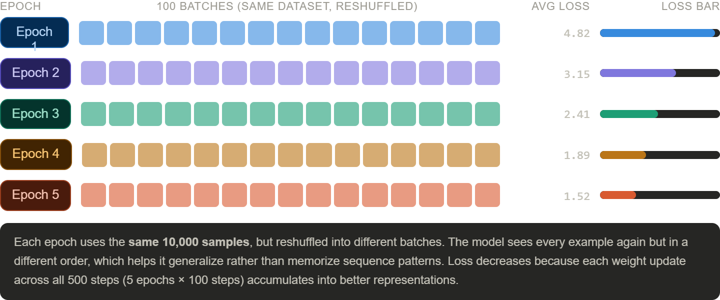
Each epoch uses the same 10,000 samples — but re-shuffled into different batches.
The model sees every example again, but in a different order. Why does this matter?
Because the model’s weights update incrementally. In epoch 1, a particular sentence might appear in batch 37. In epoch 2, it might appear in batch 12 — preceded and followed by entirely different examples. The gradient computed for that sentence will be different because the model’s current state is different, and the surrounding batch is different.
This means each pass through the data extracts different signal from the same examples. The model doesn’t just memorize a fixed sequence pattern — it builds representations that hold up across different orderings and contexts. That’s what generalization looks like at the training level.
Loss decreases because each weight update across all steps accumulates into better representations. Early epochs produce large loss drops. Later epochs squeeze out finer adjustments as the model approaches a local minimum in the loss landscape.
Concrete Numerical Example
Dataset: 10,000 sentences
Batch size: 100
Number of batches: 100
Epochs: 5
Total steps: 500
| Epoch | Steps this epoch | Cumulative steps | What changes |
|---|---|---|---|
| 1 | 100 | 100 | Weights initialized → first signal |
| 2 | 100 | 200 | Same data, different order → refines representations |
| 3 | 100 | 300 | Loss curve flattening — larger patterns learned |
| 4 | 100 | 400 | Fine-grained adjustments |
| 5 | 100 | 500 | Training run complete |
After 500 steps: the model has seen every sentence 5 times across 5 different orderings. The weights have been updated 500 times. Each update was the result of a full forward + backward pass through all model layers.
Quick Reference
Key Takeaways
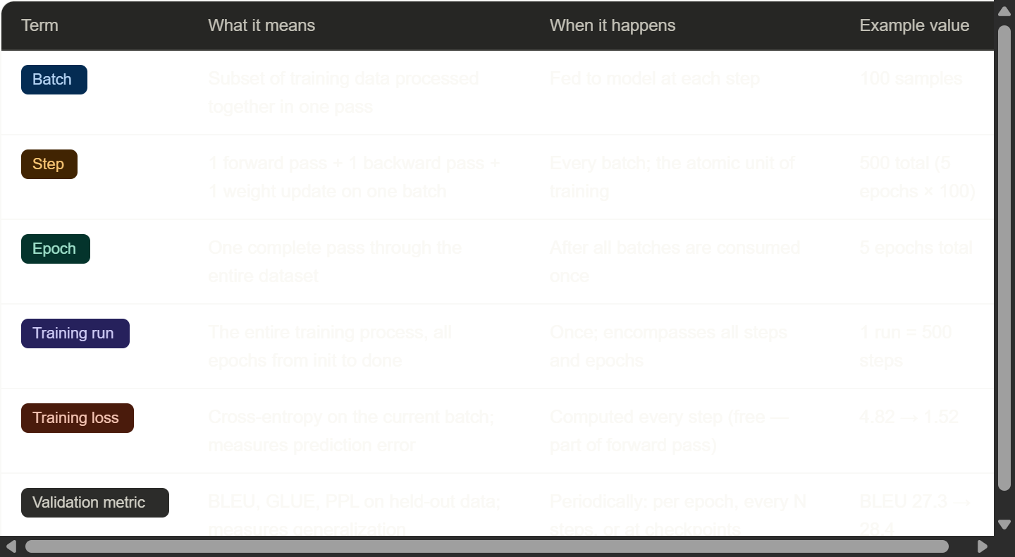
- Batch — subset of data that fits in GPU memory; processed together in one forward/backward pass
- Step — one forward pass + loss computation + backward pass + optimizer update; one weight update
- Epoch — one full pass over the entire dataset; N batches = N steps
- Training run — all epochs combined; total steps = batches × epochs
- A single step passes through all N layers of the model — forward and backward
- Adam maintains per-parameter moment estimates; it adapts the update magnitude, not just the direction
- Shuffling between epochs forces generalization — the model sees the same data but in a different context each time
- Vanishing gradients are addressed by residual connections and layer normalization, not by reducing depth
- GPU memory limits (32 GB on the V100 in 2018) are why batching exists — it’s a hardware constraint, not a design choice
Conclusion
Training a transformer is not magic. It’s a structured loop: chunk the data, run each chunk through all layers of the model, measure the error, propagate gradients backward through every layer, update every weight, repeat.
The vocabulary of batches, steps, and epochs is the vocabulary of that loop. Once you have it, everything else — learning rate schedules, gradient accumulation, distributed training across hundreds of GPUs — is just a variation on the same underlying mechanics.
The weights get nudged. Over 500 steps, those nudges compound into a model that has learned something real.