Mastering LLM Inference Optimization: KV Caching, Attention, Parallelism, and the Memory Wall
Stacking transformer layers enables the creation of large language models with billions of parameters, driving higher accuracy, strong few-shot learning, and even near-human emergent capabilities across diverse language and downstream tasks. However, these foundational models are costly to train and remain both memory- and compute-intensive at inference time, leading to ongoing operational expenses.
Modern LLMs now scale to hundreds of billions—and increasingly trillions—of parameters. Many applications require processing long input contexts, further increasing cost. In retrieval-augmented generation (RAG) pipelines, injecting large volumes of information into the model input amplifies this burden, as the LLM must process significantly more data per query.
Developers can also explore these inference optimization techniques using open NVIDIA and community models—such as the Nemotron 3 family of open models—running on the open-source TensorRT-LLM library, available on GitHub. This makes it possible to experiment with real-world inference tradeoffs using production-grade code rather than abstract examples.

Understanding LLM Inference
Large language models are typically decoder-only architectures. Most widely used models—such as GPT-3 and LLaMA—are pre-trained using a causal language modeling objective, meaning they learn to predict the next token in a sequence. Given an input sequence of tokens, the model generates subsequent tokens autoregressively, continuing until a stopping condition is met or a special end-of-sequence token <end> is produced.
This generation process can be divided into two key phases: the prefill phase and the decode phase.
Prefill Phase — Processing the Input
In the prefill phase, the LLM processes the input tokens to compute the intermediate states (keys and values), which are used to generate the “first” new token. Each new token depends on all the previous tokens, but because the full extent of the input is known, at a high level this is a matrix-matrix operation that’s highly parallelized. It effectively saturates GPU utilization.
Decode Phase — Generating the Output
In the decode phase, the LLM generates output tokens autoregressively one at a time, until a stopping criteria is met. Each sequential output token needs to know all the previous iterations’ output states (keys and values). This is like a matrix-vector operation that underutilizes the GPU compute ability compared to the prefill phase.
The speed at which the data (weights, keys, values, activations) is transferred to the GPU from memory dominates the latency—not how fast the computation actually happens. In other words, this is a memory-bound operation.
Many of the inference challenges and corresponding solutions featured in this post concern the optimization of this decode phase: efficient attention modules, managing the keys and values effectively, and others.
Batching
The most straightforward way to improve GPU utilization and throughput is batching. When multiple requests share the same LLM, the cost of loading model weights into memory is amortized across those requests. Sending larger batches to the GPU allows better use of available compute resources.
However, batch size cannot be increased indefinitely—beyond a certain point, memory limits are exceeded due to factors like KV cache growth and overall model memory requirements.
Traditional (static) batching is often inefficient in this setting. Each request in a batch may require generating a different number of tokens, leading to uneven execution times. As a result, all requests must wait for the slowest one to finish, and this inefficiency worsens when there is high variance in output lengths.
To overcome this limitation, in-flight batching is used. This technique dynamically schedules and processes requests, allowing more efficient utilization of compute resources without forcing all requests to complete together. Open-source runtimes such as NVIDIA TensorRT-LLM support in-flight batching and include optimized scheduling mechanisms for models like LLaMA and NeMo Tron, eliminating the need to build custom schedulers or low-level CUDA kernels.
Key-Value Caching
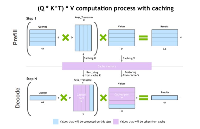
One common optimization for the decode phase is KV caching. The decode phase generates a single token at each time step, but each token depends on the key and value tensors of all previous tokens—including the input tokens’ KV tensors computed at prefill, and any new KV tensors computed until the current time step.
To avoid recomputing all these tensors for all tokens at each time step, it’s possible to cache them in GPU memory. Every iteration, when new elements are computed, they are simply added to the running cache to be used in the next iteration. In some implementations, there is one KV cache for each layer of the model.
LLM Memory Requirement
In effect, the two main contributors to the GPU LLM memory requirement are model weights and the KV cache.
- Model weights: Memory is occupied by the model parameters. As an example, a model with 7 billion parameters (such as Llama 2 7B), loaded in 16-bit precision (FP16 or BF16) would take roughly
7B × sizeof(FP16) ≈ 14 GBin memory. - KV caching: Memory is occupied by the caching of self-attention tensors to avoid redundant computation.
With batching, the KV cache of each of the requests in the batch must still be allocated separately, and can have a large memory footprint. The formula below delineates the size of the KV cache, applicable to most common LLM architectures today.
Size of KV cache per token (bytes) = 2 × num_layers × (num_heads × dim_head) × precision_in_bytes
The first factor of 2 accounts for the K and V matrices. Commonly, the value of (num_heads × dim_head) is the same as the hidden_size (or dimension of the model, d_model) of the transformer. These model attributes are commonly found in model cards or associated config files.
This memory size is required for each token in the input sequence, across the batch of inputs. Assuming half-precision, the total size of KV cache is:
Total KV cache (bytes) = batch_size × sequence_length × 2 × num_layers × hidden_size × sizeof(FP16)
For example, with a Llama 2 7B model in 16-bit precision and a batch size of 1, the size of the KV cache will be:
1 × 4096 × 2 × 32 × 4096 × 2 bytes ≈ 2 GB
Managing this KV cache efficiently is a challenging endeavor. Growing linearly with batch size and sequence length, the memory requirement can quickly scale. Consequently, it limits the throughput that can be served, and poses challenges for long-context inputs. This is the motivation behind several optimizations featured in this post.
Scaling Up LLMs with Model Parallelization
One way to reduce the per-device memory footprint of the model weights is to distribute the model over several GPUs. Spreading the memory and compute footprint enables running larger models, or larger batches of inputs.
Model parallelization is a necessity to train or infer on a model requiring more memory than available on a single device, and to make training times and inference measures (latency or throughput) suitable for certain use cases. There are several ways of parallelizing the model based on how the model weights are split.
Note on Data Parallelism: Data parallelism is also a technique often mentioned alongside the others listed below. In this approach, weights of the model are copied over multiple devices, and the global batch size of inputs is sharded across each of the devices into microbatches. It reduces the overall execution time by processing larger batches. However, it is a training-time optimization that is less relevant during inference.
Pipeline Parallelism
Pipeline parallelism involves sharding the model vertically into chunks, where each chunk comprises a subset of layers that is executed on a separate device. The model is sequentially partitioned and a quarter subset of all layers are executed on each device (in a four-way setup). The outputs of a group of operations on one device are passed to the next, which continues executing the subsequent chunk.
\(F_n\) and \(B_n\) indicate forward and backward passes respectively on device \(n\). The memory requirement for storing model weights on each device is effectively quartered.
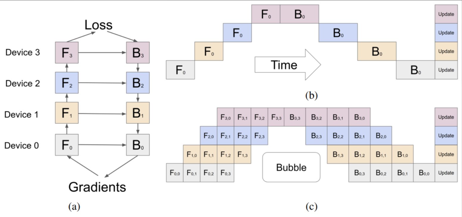
The main limitation of this method is that, due to the sequential nature of the processing, some devices or layers may remain idle while waiting for the output (activations, gradients) of previous layers. This results in inefficiencies or “pipeline bubbles” in both the forward and backward passes.
Microbatching can mitigate this to some extent. The global batch size of inputs is split into sub-batches, which are processed one by one, with gradients accumulated at the end. \(F_{n,m}\) and \(B_{n,m}\) indicate forward and backward passes respectively on device \(n\) with microbatch \(m\). This approach shrinks the size of pipeline bubbles, but it does not completely eliminate them.
Tensor Parallelism
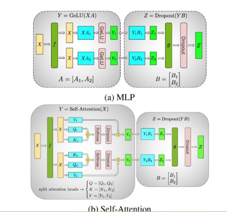
Tensor parallelism involves sharding individual layers horizontally into smaller, independent blocks of computation that can be executed on different devices. Attention blocks and multi-layer perceptron (MLP) layers are major components of transformers that can take advantage of tensor parallelism. In multi-head attention blocks, each head or group of heads can be assigned to a different device so they can be computed independently and in parallel.
Sequence Parallelism
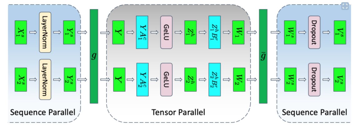
Tensor parallelism has limitations, as it requires layers to be divided into independent, manageable blocks. It’s not applicable to operations like LayerNorm and Dropout, which are instead replicated across the tensor-parallel group. While LayerNorm and Dropout are computationally inexpensive, they do require a considerable amount of memory to store redundant activations.
As shown in Reducing Activation Recomputation in Large Transformer Models, these operations are independent across the input sequence, and these ops can be partitioned along that “sequence-dimension,” making them more memory efficient. This is called sequence parallelism.
Optimizing the Attention Mechanism
The scaled dot-product attention (SDPA) operation maps query and key-value pairs to an output, as described in Attention Is All You Need.
Multi-Head Attention (MHA)
As an enhancement to the SDPA, executing the attention layer multiple times in parallel with different, learned projections of the Q, K, and V matrices enables the model to jointly attend to information from different representational subspaces at different positions. These subspaces are learned independently, providing the model with a richer understanding of different positions in the input.
The outputs from the multiple parallel attention operations are concatenated and linearly projected to combine them. Each parallel attention layer is called a “head,” and this approach is called multi-head attention (MHA).
In the original work, each attention head operates on a reduced dimension of the model (such as \(d_{model}/8\)) when using eight parallel attention heads. This keeps the computational cost similar to single-head attention.
Multi-Query Attention (MQA)
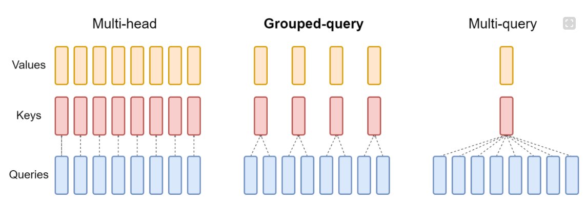
One important inference optimization for multi-head attention (MHA) is multi-query attention (MQA), introduced by Google in the Fast Transformer Decoding paper (2019). In MQA, all attention heads share the same key and value projections, while the query projections remain separate for each head, as in standard MHA.
Although the overall computation remains comparable to MHA, MQA significantly reduces memory access: the amount of key and value data read from memory is reduced to a fraction (roughly 1/number of heads). This is especially beneficial in memory bandwidth–bound scenarios, where it improves effective compute utilization. Additionally, sharing keys and values reduces the size of the KV cache, freeing up memory and enabling larger batch sizes during inference.
However, this reduction in key-value heads can lead to some loss in model accuracy. To mitigate this, models typically need to be trained with MQA from the start or at least fine-tuned with MQA enabled—often using a small fraction (e.g., ~5%) of the original training data—to adapt effectively.
Grouped-Query Attention (GQA)
Grouped-query attention (GQA) strikes a balance between MHA and MQA by projecting keys and values to a few groups of query heads. Within each of the groups, it behaves like multi-query attention.
Optimizations like MQA and GQA help reduce the memory required by KV caches by reducing the number of key and value heads that are stored. There may still be inefficiencies in how this KV cache is managed.
Flash Attention
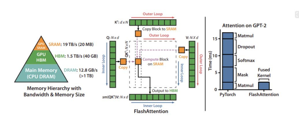
Another way of optimizing the attention mechanism is to modify the ordering of certain computations to take better advantage of the memory hierarchy of GPUs. Fusing multiple layers together during the actual computation minimizes the number of times the GPU needs to read from and write to its memory, and groups together calculations that require the same data—even if they are parts of different layers in the neural network.
Efficient KV Cache Management with Paging
At times, KV caches are statically over-provisioned to account for the largest possible input (the supported sequence length) because the size of inputs is unpredictable. For example, if the supported maximum sequence length of a model is 2,048, then regardless of the size of input and the generated output in a request, a reservation of size 2,048 would be made in memory.
This space may be contiguously allocated, and often, much of it remains unused, leading to memory waste or fragmentation. This reserved space is tied up for the lifetime of the request.

An illustration of memory wastage and fragmentation due to over-provisioning and inefficient KV cache management. Credit: Efficient Memory Management for Large Language Model Serving with PagedAttention.
Inspired by paging in operating systems, the PagedAttention algorithm enables storing continuous keys and values in noncontiguous space in memory. It partitions the KV cache of each request into blocks representing a fixed number of tokens, which can be stored non-contiguously.
These blocks are fetched as required during attention computation using a block table that keeps account. As new tokens are generated, new block allocations are made. The size of these blocks is fixed, eliminating inefficiencies arising from challenges like different requests requiring different allocations. This significantly limits memory wastage, enabling larger batch sizes (and, consequently, throughput).
Model Optimization Techniques
There are also several model optimization techniques to reduce the memory use on each GPU by making modifications to the model weights themselves. GPUs also have dedicated hardware for accelerating operations on these modified values, providing even more speedups for models.
Quantization
Quantization is the process of reducing the precision of a model’s weights and activations. Most models are trained with 32 or 16 bits of precision, where each parameter and activation element takes up 32 or 16 bits of memory—a single-precision floating point. However, most deep learning models can be effectively represented with eight or even fewer bits per value.
Reducing the precision of a model can yield several benefits:
- If the model takes up less space in memory, you can fit larger models on the same hardware.
- Quantization means you can transfer more parameters over the same amount of bandwidth, which can help to accelerate models that are bandwidth-limited.
There are many different quantization techniques for LLMs involving reduced precision on either the activations, the weights, or both. It’s much more straightforward to quantize the weights because they are fixed after training. However, this can leave some performance on the table because the activations remain at higher precisions. GPUs don’t have dedicated hardware for multiplying INT8 and FP16 numbers, so the weights must be converted back into a higher precision for the actual operations.
Sparsity
Similar to quantization, it’s been shown that many deep learning models are robust to pruning—or replacing certain values that are close to 0 with 0 itself. Sparse matrices are matrices where many of the elements are 0. These can be expressed in a condensed form that takes up less space than a full, dense matrix.
GPUs in particular have hardware acceleration for a certain kind of structured sparsity, where two out of every four values are represented by zeros. Sparse representations can also be combined with quantization to achieve even greater speedups in execution. Finding the best way to represent large language models in a sparse format is still an active area of research, and offers a promising direction for future improvements to inference speeds.
Model Serving Techniques
Model execution is frequently memory-bandwidth bound—in particular, bandwidth-bound in the weights. Even after applying all the model optimizations previously described, it’s still very likely to be memory bound. So you want to do as much as possible with your model weights when they are loaded. In other words, try doing things in parallel. Two approaches can be taken:
In-flight batching: Rather than waiting for the whole batch to finish before moving on to the next set of requests, the server runtime immediately evicts finished sequences from the batch. It then begins executing new requests while other requests are still in flight. In-flight batching can therefore greatly increase the overall GPU utilization in real-world use cases.
Speculative sampling: The basic idea of this approach is to use some “cheaper” process to generate a draft continuation that is several tokens long. Then, execute the main “verification” model at multiple steps in parallel, using the cheap draft as “speculative” context for the execution steps where it is needed.
If the verification model generates the same tokens as the draft, then you know to accept those tokens for the output. Otherwise, you can throw out everything after the first non-matching token, and repeat the process with a new draft.
Memory Hierarchy of GPUs
Memory hierarchies in GPUs are crucial for optimizing the performance of parallel computing tasks. These memory hierarchies consist of various types of memory with different characteristics to cater to the diverse requirements of GPU workloads.
| Memory Type | Size | Speed | Purpose |
|---|---|---|---|
| Register File | Per-thread (small) | Fastest | Local variables, intermediate results |
| L1 Cache / Shared Memory | KB per SM | Very fast | Inter-thread communication, data reuse within a block |
| L2 Cache | MB | Fast | Hardware-managed, reduces global memory latency |
| Local Memory | Per-thread (virtual) | Slower | Spill data when registers are insufficient |
| Texture / Constant Memory | Varies | Optimized for reads | Read-only patterns (e.g., constants, texture sampling) |
| Global Memory (VRAM) | GB | Slowest | Primary storage for model weights, activations, KV cache |
Here is a breakdown of each level:
Global Memory: The largest memory pool in a GPU, often ranging from several gigabytes to tens of gigabytes. It is accessible by all threads in a GPU, but access to global memory is relatively slow compared to other memory types. It serves as the primary storage for data that needs to be shared across multiple blocks or threads, such as input data, output data, and global constants.
Shared Memory: A smaller, faster memory pool, typically measured in kilobytes per streaming multiprocessor (SM). It is shared by threads within the same thread block. Threads can communicate and synchronize through shared memory, which is used for inter-thread communication and storing data reused by multiple threads within a block, helping to reduce memory latency.
Local Memory: Specific to each thread and usually a small cache or scratchpad memory. It is private to individual threads and is often implemented using a portion of global memory. Local memory stores temporary variables or spill data when there is insufficient register space for a thread’s variables. Accessing local memory is slower than accessing registers.
Texture Memory and Constant Memory: These specialized memory types are optimized for specific read patterns. Texture memory is optimized for 2D or 3D texture fetches, while constant memory is read-only and optimized for broadcasting constants to multiple threads.
Register File: Each thread in a GPU has access to a set number of registers—the hierarchy’s fastest and most private memory, storing local variables and intermediate results. Minimizing register usage and maximizing register reuse is essential for achieving high GPU performance.
L1 and L2 Cache: Hardware-managed caches that store frequently accessed data to reduce memory latency. Caches help accelerate memory access by storing data that threads access frequently, improving overall performance.
GPU memory hierarchies can differ between GPU architectures and manufacturers. GPU programming models such as CUDA or OpenCL allow developers to manage data movement and optimize memory access to exploit these hierarchies effectively for different workloads.
The Memory Wall and Operator Fusion
What we are describing is a fundamental challenge in computer architecture known as the “Memory Wall.” In modern computing, the speed at which a processor (CPU or GPU) can perform math has far outpaced the speed at which data can be moved from main memory (RAM/VRAM) to the processor.
When a neural network is executed “layer by layer,” the hardware often spends more time waiting for data to travel than it does actually performing the calculations.
The Memory Hierarchy Problem
To understand this, look at the “distance” between where data lives and where it is processed. Think of it like a kitchen:
- Registers/L1 Cache (The Cutting Board): Tiny capacity, but nearly instantaneous access.
- L2/L3 Cache (The Countertop): Medium capacity, very fast.
- Main Memory/VRAM (The Pantry): Huge capacity, but you have to “walk” there to get anything.
In a traditional sequential implementation:
- Layer 1: The processor fetches data from the Pantry (RAM), brings it to the Cutting Board (Registers), performs a calculation (like a ReLU activation), and then writes the result all the way back to the Pantry.
- Layer 2: The processor immediately goes back to the Pantry to fetch that same data it just wrote, brings it back to the Cutting Board for the next step (like BatchNorm), and writes it back again.
This “Round Trip” to main memory is the performance killer.
Operator Fusion: “Doing More with What You Have”
The phrase “doing more calculations on values already brought into the higher levels” refers to Operator Fusion.
Instead of treating every mathematical operation as a separate step that requires saving and loading, a compiler (like XLA or PyTorch Inductor) will “fuse” multiple layers into a single kernel.
The Sequential Approach (Suboptimal):
# Each line here is a round-trip to main memory
x = matrix_multiply(input, weights)
x = relu(x)
x = batch_norm(x)
The Fused Approach (Optimal):
The processor loads the data once and performs all three operations while the data is still sitting in the Registers or L1 Cache.
Load data → Multiply → ReLU → BatchNorm → Write result
By doing this, you maximize Arithmetic Intensity—the ratio of math operations performed per byte of data moved.
Why Fusion Isn’t Always the Default
If fusing layers is so much faster, why do we describe them as separate layers?
- Modularity: It is much easier for humans to design, debug, and swap layers if they are discrete blocks.
- Memory Constraints: Some operations (like large convolutions) produce so much intermediate data that it physically cannot fit into the high-level caches all at once.
- Hardware Specifics: Every GPU and CPU has different cache sizes. A fused kernel that works perfectly on an NVIDIA H100 might “spill” out of the cache on a smaller mobile chip, actually making it slower.
When people say it’s better to do more calculations in the “higher levels of the memory hierarchy,” they mean: stop moving data back and forth to RAM. If you’ve gone through the “expensive” effort of fetching a piece of data into the processor’s immediate workspace (L1/Registers), you should squeeze every possible calculation out of it before letting it go.
Key Takeaways
- Prefill vs. Decode: Prefill is compute-bound (matrix-matrix ops, saturates GPU); decode is memory-bound (matrix-vector ops, bottlenecked by bandwidth).
- KV Caching: Avoids recomputing attention keys/values; scales linearly with batch size and sequence length — the primary memory bottleneck at inference time.
- Batching: Static batching wastes GPU resources on variable-length sequences; in-flight batching dynamically fills gaps to maximize throughput.
- Pipeline Parallelism: Shards layers across devices, reducing per-device weight memory; introduces pipeline bubbles mitigated by microbatching.
- Tensor Parallelism: Shards individual layers horizontally (attention heads, MLP weights); enables true parallel computation across devices.
- Sequence Parallelism: Extends tensor parallelism to ops like LayerNorm and Dropout by partitioning along the sequence dimension.
- MQA / GQA: Reduce KV cache size by sharing key-value heads across query heads; MQA is aggressive (one K/V head), GQA is a tunable middle ground.
- Flash Attention: Fuses the attention computation into a single kernel using tiling; avoids materializing the full attention matrix in HBM.
- PagedAttention: Manages KV cache blocks non-contiguously (inspired by OS paging); eliminates fragmentation and over-provisioning, enabling larger batch sizes.
- Quantization: Reduces weight precision (FP16 → INT8 or lower); smaller memory footprint, higher effective bandwidth, potential accuracy tradeoff.
- Sparsity: Pruning weights close to zero; structured 2:4 sparsity has native GPU hardware support; combinable with quantization.
- Speculative Sampling: Uses a cheap draft model to generate candidate tokens; verifies them in parallel with the large model; accelerates latency without changing output distribution.
- The Memory Wall: The gap between compute speed and memory bandwidth is the dominant bottleneck; operator fusion is the primary tool to bridge it by maximizing arithmetic intensity.
Conclusion
LLM inference is not a single bottleneck — it is a stack of overlapping constraints across compute, memory bandwidth, memory capacity, and scheduling.
The decode phase is memory-bound by nature. KV caching trades memory for speed, but the cache itself becomes the new bottleneck at scale. Parallelism strategies spread the load across devices but introduce communication overhead. Attention variants like MQA and GQA shrink the KV footprint. Flash Attention and PagedAttention address how that memory is accessed and managed. Quantization and sparsity compress the weights. Serving techniques like in-flight batching and speculative decoding maximize hardware utilization at the system level.
Understanding which layer of the stack is the bottleneck in a given deployment—and which optimization addresses it—is the core skill in LLM inference engineering. The Memory Wall is real, and every technique in this post is, in some form, a strategy for working around it.
Tools and Frameworks
- NVIDIA TensorRT-LLM — Production-grade inference library with support for in-flight batching, quantization, and fused kernels.
- NVIDIA Megatron-LM — Framework for large-scale model training and parallelism (pipeline, tensor, sequence).
- NVIDIA NeMo Framework — End-to-end platform for building, training, and deploying LLMs at scale.